Regulators can dull, but never declaw GenAI due to Moore’s law

01 Jan 2024

“AI” has been the Wall Street Journal’s darling buzzword of the past year. If there’s any one topic their technology section loves to cover, it’s how FAANG/MAMAA/Magnificent 7 will break the world selling their “AIs” to every business imaginable, or how Elon Musk claims those “AIs” will lead to our doom. I can practically feel the business people salivating every time they hear of a new profitable technology. But I realize it’s time to revisit whether we should actually ready our pitchforks and torches. There’s a clear divide between people who understand the theory behind the technique, and people who invest a jaw dropping amount of money into the former. This is unfortunate, because the theory will be very useful knowledge when the consequences start popping up like whack-a-moles.

Even Google’s CEO unironically proclaimed that “AI will be more impactful to humanity than fire or electricity.” How convenient for someone with 227K shares in a company that claims itself at the frontier of AI to chum the investor tank… Fire provided light and warmth, a lethal weapon against lions, and newly digestible foods. Electricity amplified human effort to the limit of energy, increasing quality of life for everyone. These two inventions were game changers for the trajectory of humanity. In comparison, generative AI seems like a neat party trick, a proof of concept for something bigger. Yet, I invite you to read the lyrics of the Gershwin classic, “They All Laughed.” Generative AI amplifies human communication to the limit of creativity, a truly potent but double edged sword. It will certainly push content moderation past its limits, ruin the creativity and dignity of countless people, even destroy the integrity of information itself, and there’s nothing the world can do about it except stop making better computers. Let me explain.

Part 1: Generative AI is still just approximation

To understand the potential of the technology and why we should be careful, we have to attack it from different perspectives. Plus, I feel like there are many misconceptions surrounding AI and ML propagated both inside and outside the community. Like I mentioned, the media is incredibly bullish yet fearful of its future, predicting everything from a work-free utopia to a robot-dominated Orwellian dystopia. Even practitioners on Reddit and Stack Exchange frequently confuse the purpose and theory behind the methods. I once read someone on Reddit saying linear regression fits an arbitrary function to classify data. Both linear and regression are literally in the name… But the field is really just a diverse kitchen sink of problems. Each domain’s textbook provides a different perspective on those problems, but consolidating them all together yields the bigger picture. A cognitive psychology textbook explains the brain’s approach, a statistics textbook explains hypothesis testing and numerical methods, a deep learning textbook explains teaching neural networks, while a philosophy textbook explains the pursuit of truth. They all tell a different side of the same tale of approximation, but they’re split across different years of education and have their own nomenclature. Thus, let’s connect all the important concepts by breaking down large ideas to fill any gaps.

The cognitive psychology approach

Artificial intelligence is the expression of statistics and logic through algorithms to make machines that exhibit intelligent characteristics. This definition is intentionally vague, because the sheer notion of “intelligence” is ethereal. There are multiple fields of psychology and science dedicated to understanding this concept. Let’s start with the cognitive psychology approach. The most applicable way I can think to consolidate them is “combining prior knowledge with hints from the input to solve problems.” This is the combination of top-down and bottom-up processing, the two primary approaches your brain uses for sensation and perception. Of course, achieving this level of processing requires:

• Memory, to store past stimuli in both a short-term working directory and a long-term knowledge bank, with mechanisms to retrieve and to forget
• Learning, to adapt through conditioning and observation to populate that knowledge bank
• Problem solving, to overcome obstacles in situations through pattern recognition and critical thinking
• Decision making, to react to situations appropriately through heuristics and to consolidate complex thought into an output.

But there is a good reason for this complex set of primitives. They allow us to reason through a diverse set of situations using a limited toolset, meaning they’re composable. Consider the problem of finding the shortest path between two points in a maze. Compare two strategies to pick the next point (aka vertex) to visit.

1. Always choose the next vertex closest to the start (Dijkstra/UCS).
2. Always choose the next vertex closest to both the start and end-goal (A*).

Both approaches implicitly use hints from the input through the triangle inequality, that AB + BC > AC if B is not along the shortest path. Yet the first one isn’t considered intelligent because it chooses the best action only for the short term, without leveraging any prior knowledge to get to the answer faster. Meanwhile, the second one estimates the distance to the end-goal using a heuristic, and minimizes that distance quickly yet cheaply. A* is a small modification over Dijkstra’s, yet the inclusion of intelligent decision making helps it find the optimal solution much faster.

Figure 1.1. Uniform cost search (left) expands significantly more vertices than A* search (right) to find the shortest path.

A* is an example of a machine that behaves rationally, because it chooses the best option at every turn. But the field of graph search is very much a tiny subset of AI. Though artificial intelligence is quite an enormous discipline, two abstract properties of any solution are how much action it requires and how much rationality is desired. Therefore, you can chart the field using quadrants to reason about the nature of problems.

Accordingly, machines that behave humanly act in a way that emulates understanding of human emotions and social context. For example, social robots, video game NPCs, and ChatGPT try to imitate human behavior, even if they don’t internally function that way. Machines that behave rationally act in a way that maximizes utility, but whether that’s for the good of the user or society is open for interpretation. For example, self-driving cars, smart energy grids, and stock trading algorithms make the optimal decision at every turn. These problems all have something significant in common; the correct answer is influenced by a lot of variables and is therefore difficult to find, but a good-enough answer can be approximated using fewer variables.

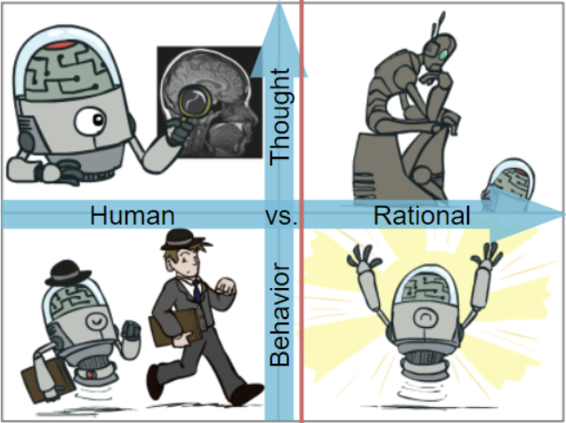
Figure 1.2. Artificial intelligence is divided into 4 quadrants based on the desired amount of action and rationality.

The philosophical approach

To understand the theory of approximation, we can turn to a thought experiment from 1990 that explains universal truth using particle physics, Laplace’s demon. Under the classical model of physics, if you know the current position and velocity of all particles in a system, then you can calculate the positions and velocities of any past and future time. This property applies from a simple two-particle system all the way to the entire observable universe, and holds because of conservation of energy. In other words, the state of the world changes in a predefined sequence (deterministic) and we can model and calculate these numbers (computable) given all positions and velocities at a single time (observable). A demon with unbounded knowledge could know such information about every particle, then it could answer any question with perfect accuracy. It could predict the weather 5 years from now, tell you every election result, plus how many of them will be manipulated. We can in fact model the demon as a function f(x1, x2, …, xN) -> y1, y2, …, yN, where each xi and yi represent particles. It takes in input one state of the universe and tells you the next. But the world is chaotic, and small phenomena can have huge consequences because of the butterfly effect. As soon as you start getting rid of variables, maybe leaving out some particles here and there, you lose potentially important interaction terms, and the model is no longer perfectly correct. What if that missing particle hits some atom in my brain in a certain way that compels me to buy Sony XM4s instead of XM5s? Then the demon is no longer perfectly accurate, but rather an approximation, a good-enough answer.

Laplace’s demon is a useful thought experiment because it shows the upper bound on the dimensionality of real world functions; they are discrete due to the atomicity of particles, and have finite domain and range because the speed of light is fixed. It’s clear that this logic applies to such functions of any dimensionality. In fact, it follows that every real world trend or phenomena is a deterministic function mapping f(x1, x2, …, xN) -> y1, y2, …, yM, where N,M <= particles in the universe. Now for convenience, let’s rewrite x1, x2, …, xN as a vector, X, an arrow in N-dimensional space, so now our functions are f(X) -> (Y). Our practical problem is we can’t possibly compute such a complex function using real computers. It’s too high dimensionality, and we must somehow reduce the number of variables to something we can handle easier. Let’s take a quick digression to probability to alleviate this problem. How do we know which variables we can safely overlook? We can only overlook some variables under an assumption of conditional independence. Once you know the values of the significant independent variables, then knowing the dependent variable doesn’t tell us anything about the “insignificant” or noisy independent variables. This is because there is little, maybe even no influence between the output and noise. But this also means when none of the variables are insignificant, then there is no way to approximate the function to any extent. A clear cut example of this “random” distribution is XOR: f(x, y, z) = x XOR y XOR z. If you know x = 1, then even if you know f(x, y, z) = 0, you haven’t learned anything about y or z. Even scaled up to millions of inputs, there is no way to approximate this function with less variables at all. In terms of information, these functions have maximum entropy with no redundancy.

Figure 1.3. XOR of k variables cannot be approximated with less than k parameters.

Luckily, real world trends are often explained by significantly less variables than go into the whole equation. That’s a good thing because though tomorrow’s weather may be a chaotic function of some quadrillion variables representing particles in the atmosphere, I still need to know whether to pack an umbrella. If the underlying distribution takes a set of parameters, X, we can partition them into two sets, (X’, E), where X’ are the k most important variables, and E are the rest. The important k variables capture most of the variance, or the way the distribution changes with inputs. The number of selected variables, k, depends on how much of this variance we wish to capture and how many dimensions we’re comfortable dealing with. This process is called feature selection, which we do implicitly when thinking about complex distributions (feature is our measurement of an underlying variable). When I consider the likelihood of eating at Chick-fil-A, I’m probably just thinking about my hunger level and distance to the nearest one, not the restaurant’s Yelp rating or the amount of fuel in my car. This conditional independence between insignificant variables is notated as P(f(x) | x, e) = P(f(x) | x); we can comfortably forget about e. This property has significant implications, and indeed it is what enables approximation. There are functions in lower dimensions that still capture most of the variance of more complex functions. We call these lower-dimension functions approximators or models. The rest of the variables are more like noise: essential for a perfectly accurate answer, but can be overlooked to capture the heart of the problem. It’s just like the saying, “if you can’t explain it simply, you don’t understand it well enough.” This saying itself models the idea behind the theory of approximation. How cool is that!

We’ve established that approximation is capturing maximum variance using minimum variables. Back to our A* search example, the heuristic approximates the true distance from the goal state, which otherwise takes a long time to compute. If the true distance was a function, it might consider every vertex in the graph, while the heuristic would just consider the start and goal positions. In function notation, the true distance from s to t is dist(s, v1, v2, …, vN, t), where N = |V| - 2, while the heuristic is just h(s, t). Note that this notation is the same as f(x, y, z, …, w) multivariable calculus. If you’re used to programming, this might not seem like a big deal because those extra variables could just go unused. But think about the domain visually: the number of axes increases with every additional parameter, which causes the domain to grow exponentially. However, adding another parameter rarely “populates” the range at an equivalent rate, making the domain sparser and sparser with more parameters. This is fine if you know the closed-form definition of the function, like y = mx, but we’re often dealing with discrete distributions via observations. As the distribution’s domain gets sparser and sparser, you need exponentially more observations for the same density, or resolution of information. If we keep the same number of observations, our models will likely overfit the data points and just match them exactly instead of learning the true distribution, like pulling a string taut through a small set of holes. This problem is the curse of dimensionality.

Figure 1.4. Volume increases exponentially on the number of dimensions, causing the density of observations to decrease exponentially on the number of parameters.

The optimization approach

The curse of dimensionality is the arch nemesis of approximation, giving us a huge incentive to keep our approximator function as simple as possible. Computer scientists fear exponential growth because we like both letting the domain be unbounded, and evaluating our functions in a reasonable time. Exponential functions do not allow these two properties to coexist because their growth accelerates, or increases multiplicatively, whereas polynomials increase additively. That’s why the A* heuristic function h ideally doesn’t take any intermediate points as parameters. But this heuristic requires some strong assumptions of dist, which is that s and t are really good indicators of the true distance. What do you do if the true distribution is too complex to know such a trick about? What if all you have are some (X, y) pairs at specific points? One incredibly successful method to find this good-enough answer using a set of observations is to tune some simple function to fit a more complex function. This statistical technique is called supervised learning. The enormous success of supervised learning has caused solutions from the behavioral half of AI to become integral to our daily lives.

Figure 1.5. A set of observations (purple) initially approximated by the hypothesis parabola, y = x^2 + x + 1 (blue).

For example, let’s say I have black-box function f. I don’t know what it is, but I can evaluate it at arbitrary points. So I did that to produce 30 observations, (0, 4.2), (1, 7.9), (2, 12.4), (3, 21.7), … (29, 1687.3). From initial thoughts, maybe from domain knowledge, this seems like a quadratic relationship between x and f(x). So let’s start with the general quadratic equation, g(x) = ax^2 + bx + c, and figure out the 3 coefficients, a, b, and c, that minimize the difference between our prediction and the given answer. There are an infinite number of real valued parabolas, and each one is a hypothesis that we think could explain the data. Thus we need to search for the hypothesis that explains the data the best. It doesn’t matter which hypothesis we start with, so let’s pick (1, 1, 1). Our initial predictions are thus (0, 1), (1, 3), (2, 7), …, (29, 871); quite far off, but we’re on the right track. Our goal is to find the values of coefficients that minimize the difference between my predicted g(x) and the f(x) from the observations. In other words, Our task is finding some parameters that model a distribution, given a set of (feature, class) observations. In this case, we have 1 feature, x, and 1 class, y. The number of features is the dimensionality of the dataset, and the number of observations is the size. By running supervised learning on our model given the observations, we can figure out that the underlying distribution is y = 2x^2 + 4 with some random noise. That means the best hypothesis was (2, 0, 4). Note that “evaluating a black-box function” is exactly what surveys, real-world measurements, simulations, and experiments fundamentally are, and fitting a simpler function to those observations is machine learning.

But there are limits to this approach depending on what kind of function we use to approximate. And we can precisely quantify this complexity-accuracy trade off using a beautiful tool we all forgot about from calculus: the Taylor series. It uses a power series polynomial to approximate any infinitely-derivable function centered around a point. But recall that a polynomial of limited degree can only approximate a higher order function for a specific interval before it diverges. Even with unlimited degree, most functions have a finite range of approximation. If the power series (approximator) converges with infinite terms, then we can directly calculate this radius of convergence using a ratio test. The idea behind Taylor series elegantly transfers to nonlinear approximators too: Fourier series globally approximate using a composition of sin and cosine, and wavelet transforms approximate using lots of small complex functions (like convolutional kernels). The key takeaways from these algorithms is that by using a more complex approximator, we increase both the accuracy and range of convergence, but nonetheless there is almost always a quantifiable limit.

Figure 1.6. Higher degree polynomials can approximate y = sin(x) more closely than lower degree.

This is a fundamental headache for machine learning practitioners. Not only does the curse of dimensionality compel us to use simple models, but even if we were to use infinitely complex models, we still couldn’t perfectly approximate functions over their whole domain. Machine learning experienced a long winter from 1987-1993 when researchers believed we couldn’t approximate useful enough real-world functions because they were too complex for our models and computers. But the computer engineers were cooking up better computers superlinearly, and the pipe dream quickly became feasible. We still needed better models than polynomials to make the most of the abundant compute and datasets. They came up with some clever techniques like progressively partitioning your inputs to reduce entropy (decision trees), and finding the high-dimensional plane that maximizes the distance between the closest points of different classes (support vector machines). They even composed many of these models in parallel (bagging) and series (boosting), because combining many simpler models stochastically makes the most of our limited data.

But one architecture in particular proved to be versatile to a whole new extent. It combined linear regression with a nonlinear function sandwiched between each line. Try to visualize it in your head: the composition of two lines is just another line. The composition of 20 lines is still just a line. But add some non-linearity between each function, and it can take literally any shape over any range. As it turns out, this idea was the recipe to the most robust approximating function, the neural network. There’s a fundamental difference between neural networks and other models: a sufficiently complex neural network can approximate any real valued function over its entire domain. This technique bypasses the limit of polynomials explained by Taylor series, and of sinusoidal functions explained by Fourier series. Indeed, researchers formulated elegant proofs for the approximative capabilities of this architecture, called universal approximation theorems. Two theorems in particular gave a formal justification for the field of deep learning:

1. Any feedforward neural network (DAG) with sufficient width can approximate any continuous function for any sized interval
2. Any recurrent neural network (directed cyclic) with sufficient width can approximate any dynamical system for any set of states

We’ve talked about models a lot so far, while assuming we know the likeliest hypothesis (set of parameters) to expose the theoretical potential of each function. But how do we actually find those parameters, especially given our dataset size and compute limitations? By investigating Taylor series and universal approximation theorems, we’ve been operating under the decision problem, “is there a hypothesis with at most e error?” We need to reframe and solve the optimization problem, “what is the hypothesis with the lowest possible error?” Now this is a problem we can solve efficiently with algorithms like gradient descent, rather than with exhaustive search. Let’s notate the phrase “hypothesis with lowest possible error” as max h in H (P(h | E), meaning the hypothesis that best explains the data. By definition of conditional probability, note that P(h | E) = P(h, E) / P(E), which translates to “how likely is h true in the worlds where E is also true.” Note by the same property that the inverse is also true, that P(E | h) = P(h, E) / P(h). Both of these equations can help us learn by capturing different probabilities about hypotheses and data, so let’s combine them into one equation by their common term: P(h | E) = P(E | h) P(h) / P(E). This formula should be ringing bells at this point, because it’s Bayes’s rule!

The Bayesian statistics approach

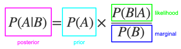
Figure 1.7. A prior belief can incorporate new information using a conditional probability.

Semantic definitions of these 4 terms helps intuit through the implications. Note that I’m substituting A with h for hypothesis, and B with E for evidence.

• Prior: How much did we believe this hypothesis before seeing the new evidence?
• Marginal: How likely is seeing this evidence across all possible hypotheses?
• Likelihood: How likely is seeing this evidence under this hypothesis?
• Posterior: How much do we believe this hypothesis in light of the new evidence?

Our objective is to explicitly model the posterior, P(h | E), and Bayes’s rule gives us the probabilistic machinery to calculate this. Starting with our current belief of this hypothesis, we incorporate the newly seen data through the ratio of the likelihood to the marginal likelihood. If this ratio is greater than 1, that means you’re likelier to see this data whenever h is true than under all possible hypotheses. Bayes’s rule is fundamentally an update step, one we take successively in order to learn. Our practical problem is that the likelihood and marginal are really difficult to model directly; how do you even answer the question “how likely is the air pressure to be 1.45atm?” Modeling the marginal is hard because it requires integrating over all possible hypotheses, and the number of hypotheses is exponential on the number of parameters. Modeling the likelihood is hard because it requires data that encompasses all variables at play; if you leave out significant latent variables, then the distribution is off even when you know when h is true. That’s why we implicitly model these two distributions together via the observation set. It’s less powerful because you can’t extract the marginal or likelihood, but combining them together is significantly easier to learn. Thus, our traditional supervised-learning approach to regression and classification problems is explicitly modeling the posterior distribution, allowing us to discriminate between different hypotheses to find the likeliest one given data.

The optimization approach we use to find P(h | E) is to formulate error as a function, L, and find the root of dL/dW with the minimum value of L. Since the hypothesis h is a set of parameters, W, dL/dW tells you how much error changes for each unit change of parameters. Recall that the roots of dL/dW correspond to maxima or minima, and in this case we’re interested in minima: the smaller the error, the better that hypothesis explains the data. But formulating an equation offline that solves this directly at once, a closed-form solution, is another victim of the curse of dimensionality. Indeed, out of all the convex and differentiable optimization functions there are, humanity only knows of an algorithm to find the best line: least squares linear regression. Instead, we can learn online and minimize the error function iteratively, updating weights in the opposite direction of the partial derivatives to guide our path. This algorithm is called gradient descent, and repeating it across all partial derivatives tells you what direction to tweak every parameter to explain the data the best! The magnitude of update is less consequential than the direction, but nonetheless the best step size naturally scales with the slope; if you’re on a steep hill, you can take a bigger step with less fear of missing the bottom than on flatter ground. Even when using an error function that includes extra terms to avoid overfitting (like regularization), the derivative remains the same given you know h’. Thus, learning P(h | E) is straightforward when h represents an elementary function, but what if the model is a composition of functions? Then you have to use the chain rule to find the derivative of the error function. And recall that neural networks are just a composition of elementary functions, so let’s explore that example.

Figure 1.8. A parameterized function can be iteratively minimized by nudging each parameter in the opposite direction of its partial derivative.

The deep learning approach

Taking the derivative of a neural network is a fascinating and strangely intuitive inductive process. For context, the network is a function f(X, L1, L2, …, Lk), where X is the input, each Li is a set of neurons whose input is the aggregated output of Li-1, and the network returns the output of Lk. Each neuron is a function g(X, W, a), where X is a k length vector of inputs, W is a k + 1 length vector of weights, a is a nonlinear function, and the neuron returns a(x dot w). But we only know what the output for layer Lk should be, because it’s the label. We can determine the error of Lk and optimize those neurons’ weights with the gradient descent algorithm described above. But this doesn’t help us refine the weights in L1 to Li-1. But recall that the input of Lk is the output of Lk-1, and the input of Lk-1 is the output of Lk-2, and this repeats inductively until you reach the original input, X. This implies that each neuron is responsible for some fraction of the next neuron’s error. And this fraction is satisfyingly simple to calculate: it’s the next neuron’s error multiplied by the corresponding weight for the previous neuron! After all, the weight represents exactly how much an input contributes to the final output. This weighted value is called the upstream gradient and is passed down to the previous layer, and for each neuron, the sum across the next layer represents how much that downstream neuron contributed to the final error. Now in order to calculate how much each individual weight contributed to this neuron’s total error contribution, we take the partial derivative dN/dW1 using chain rule. Multiply this local gradient by the upstream gradient, and we’ve just obtained the dL/dWi that gradient descent needs! Lastly, to pass the error downstream to the previous layer, we multiply this value by the corresponding weights like before. The process of using the partial derivatives with respect to weights to minimize the network’s error is called backpropagation, and is the fundamental algorithm of deep learning. This algorithm applies to RNNs as well because they can be unrolled into a DAG, producing the familiar feedforward network.

Figure 1.9. Input processing feeds forward, therefore contribution of error propagates backward due to the chain rule of Calculus.

Finally, generative AI

It’s time for the paradigm shift I mentioned at the start of the article, from discriminative to generative approximators. Luckily, the principles still follow Bayes’s rule, just with a different objective: model the joint probability, P(E, h). This enables us to generate likely (feature, class) pairs that mimic those in the training set. But modeling joint probabilities is exponentially harder than modeling conditional probabilities like P(h | E) because of the increase in dimensionality and complex interactions between these new dimensions. But recall from the definition of conditional probability that P(E, h) = P(h | E)P(E) = P(E | h)P(h). We already know P(h), our prior belief, and we know how to calculate P(h | E) through our discriminative methods from above. So generative models can take the shortcut by explicitly modeling the marginal OR likelihood distributions. Although the marginal is usually more complex than the likelihood because it involves integrating over all possible hypotheses, our choice will depend on how the learning problem is set up. For practicality, we have to use some trick to cope with this computationally difficult task. Now we have a well defined task for generative AI: explicitly model the prior and likelihood, or the posterior and marginal likelihood!

Naive Bayes models are the simplest generative approximators. They assume that the features in E are conditionally independent given the hypothesis h, which simplifies the computation of P(E | h) immensely. Under this assumption, P(E | h) can be expressed as the product of individual probabilities for each feature, because P(Ei | Ej,h) = P(Ei | h). This makes it feasible to handle high-dimensional data spaces without dealing with the curse of dimensionality directly. This method effectively utilizes the prior P(h) and the likelihood P(Ei∣h) for each feature Ei​ to compute the joint probability P(E,h). While the conditional independence assumption may not hold true in all cases, it allows Naive Bayes to perform remarkably well in many practical scenarios, especially when the dimensionality of the feature space is large.

Auto-regressive transformers are currently the most complex and robust generative approximators, but they use a trick by modeling sequences. Their key insight is to weigh the importance of each element of the input sequence with every other element at once (self-attention mechanism), which both enables long run dependencies and makes the model massively parallelizable. Transformers are a combination of self-attention mechanisms with feedforward networks, and still learn through gradient descent since self-attention is a differentiable linear function. However, I mentioned that gradient descent is used to learn P(h | E) in a supervised learning context, but generation requires modeling P(E, h), so what gives? Well, auto-regression blurs the line between h and E, and they learn the marginal and posterior simultaneously by decomposing E into a sequence of conditional probabilities. Remember how ChatGPT has to generate one token at a time to “reconstruct” the whole sequence? In this learning configuration, the hypothesis at each step is the next word, and the evidence is every word before it. There is still an (X, y) pair at every step, but y is simply the last actual token of X. So iteratively sampling from P(xn | x1, x2, …, xn-1) gives you the likely hypothesis, and together they construct the marginal, P(E). Modeling sequences is the clever shortcut that auto-regressive models use to be generative.

Figure 1.10. The marginal likelihood can be decomposed into a sequence of auto-regressive conditional probabilities.

Morals of the story

This top-down story consolidates the cognitive psychology, philosophy, optimization, Bayesian statistics, and finally deep learning perspectives on AI. You should understand that ChatGPT works under the same conceptual foundations as A* search. And I think there are two conflicting morals to this story of approximation. Together, they form the bias-variance tradeoff!

First, choose the simplest hypothesis that still explains the data. Simpler hypotheses are more interpretable and have less “holes” in their story. Conceptually, this means your story should be consistent and complete, and similar questions should have similar answers. If I ask you “why is there glass shattered on the floor” and you answer “the cat did it,” that’s fine so long as if I ask “why is the trash can lying on its side,” you don’t answer “God wanted banana peels on the floor…” This approach minimizes variance by choosing a smoother approximation. In the supervised-learning context, this translates to lower-magnitude and less parameters, like the line (2, 0, 4) over the line (10, -3, 13, 7), such that small changes in input don’t radically change the output. This is important because humans are merely agents in a partially observable environment, and as such our observations are limited and skewed. Choosing a simpler hypothesis makes the most of your observations by learning the trend instead of the points, just like believing in coincidences over ghosts. This simplicity-bias is colloquially known as Occam’s razor.

Second, choose a hypothesis that is complex enough to actually model the underlying trend. Complex hypotheses can capture the root cause of phenomena when simple assumptions are insufficient or dangerous. By definition, supervised-learning is a dumb optimization algorithm that finds correlation between evidence and hypotheses. The simplest hypothesis that explains the data is usually a correlative relationship, not a causative one. This is precisely why models predict that being black or Muslim makes you more dangerous than being white, and being a woman makes you less suited for male-dominated careers. There are certainly such correlative relationships in our datasets, but relationships do not attempt to explain the true underlying distribution. This behavior is indicative of a naive or low-dimensional hypothesis. In the supervised-learning context, a potential solution is higher-magnitude and more parameters, such that the model can learn the nuanced trend responsible for the observations. This approach minimizes bias (aka error) by choosing a better explanation for the evidence. Balancing the preference for simplicity with the preference for causation birthed the field of AI Ethics & Safety.

Finally, as people making models that can have a significant impact on the consumer’s life, it is our responsibility to stay vigilant of such dangerous correlations and stay skeptical of highly accurate yet simple models. But I didn’t agree with this sentiment for a long time for the same reason I would take money from a lost wallet: if I don’t do it, someone else will. Caring about AI safety is generally at odds with performance, which is lethal in such a competitive and fast paced market. Free market forces should surely prefer companies that move fast and break things, right? But safety has tangible financial value, from a lucrative avenue for marketing to avoidance of potential lawsuits down the line. There is a third axis in the tradeoff space of models, which is alignment with good human ethos. But whether companies actually do this hard work before plastering “We care about AI safety!” on their websites is another story…

Part 2: But approximation knows no bounds because of accelerating compute and data availability

That was just the theoretical story of approximation. Here on Earth, we are practically limited by the speed/memory of computers and the quality/quantity of observations. So it’s only natural to assume that our innocent dream will face a disappointing wakeup when brought to the real world; after all, all ice cream cones melt and all bubbles pop. I mentioned that machine learning faced a long winter in the 70s because our models couldn’t approximate useful real world phenomena. Their limitation was that “advancements in the size, complexities, and hyperparameters for deep neural networks significantly outpaced research in semiconductor technology that is core to any hardware system” (Waterloo Business Review). Complex functions require more parameters to approximate, but the curse of dimensionality made this computationally unfeasible. Still, humanity’s hunger for functions to approximate is exponentially growing, and we want Star Trek now! Semiconductor research is what brought us out of that first winter, and persistent innovation is what will keep us out.

Next, I will prove that you do have sufficient resources (data, compute, time) through 5 trends in data collection and computer engineering. I will also show that these trends are sustainable due to their exponential nature, which enables this property for the foreseeable future.

Trend 1: The number of transistors in a computer is increasing exponentially with time. The speed of computer processors caught up to the expensive demands of deep learning, owing to the ingenuity of electrical and computer engineers. Gordon Moore picked up on this trend and modeled it as “the density of transistors will double every 18 months.” Astoundingly, his approximation converged to the real world distribution of transistor density for nearly 3 decades.

Figure 2.1. Single-CPU transistor density increased exponentially, but it has slowed to polynomial growth since 2005. Yet, the total number of transistors continues to increase exponentially due to the many-core trend (ResearchGate).

But why should software engineers care about transistor density in the first place? In other words, what is the relationship between transistor density and speed of applications? It comes down to the clock speed and throughput of CPU instructions. Keeping transistors closer together means you can fit more of them on the same sized chip, which has 3 benefits:

1. Faster clock speed: The propagation and wire delays within physical logic circuits get smaller. This latency is already miniscule owing to the speed of electrons, but when each clock tick takes less than a billionth of a second, this is the limiting factor.
2. Higher instruction throughput: Having more transistors means you can do more each clock cycle. The microarchitecture can alleviate structural hazards, or when two instructions in the pipeline contend for the same resource, by having more total resources (ALUs, registers, cache).
3. Less electricity consumption: Transistors take electricity to activate their output (gate-capacitance), and the resistance generates heat. But smaller transistors have smaller gate-capacitance, which means you can scale them up without paying the energy price.

These effects cause processor throughput to increase linearly with transistor density, and transistor density increased exponentially with time. This trend is largely what enabled approximators to achieve previously unimaginable results, because the cost of operation reduced exponentially. In other words, the performance of supervised learning scales with computational power. However, the graph above has another key feature: single-CPU performance is only increasing polynomially as of 2005 (we’ll get into why transistor count is still exponential shortly). If processor throughput were to continue to increase polynomially, then that would have dramatic impacts on the future of approximation, because supply would not keep up with demand. There are two insurmountable reasons why supervised learning is a computationally expensive problem:

1. Dataset size: The required number of parameters is logarithmic on the complexity of the underlying trend - if there is twice as much information in the function, then it takes one more parameter in a binary encoding. However, the required number of observations is exponential on the number of parameters due to the curse of dimensionality, causing the required number of observations to be polynomial on the complexity of the underlying trend.
2. Convergence time: The required number of iterations of gradient descent is polynomial on the number of parameters. This is because in every iteration, the derivatives must be computed for every parameter, and they must all be optimized to minimize the error function.

Luckily, both of these reasons are polynomial, meaning deep learning is not NP-hard. As long as CPU speed kept increasing exponentially due to transistor density, this was fundamentally OK because we could brute force our problems. But now that single processor speed is only increasing polynomially, the overall increase of model accuracy should only increase polynomially as well! This will not do because we are hungry for better models.

But don’t base your assumptions on a single graph. Let’s investigate why Moore’s law is dead through solid-state physics! First, we need to discard all of our abstractions. Computer scientists can talk about logic all they want, but to implement it in the real world, we need a material that can encode multiple states. And to encode multiple states, the material must measurably change on an input. Ideally, the thing should be deterministic, easily measurable, and easily changeable. I could theoretically build a computer made of thermometers that measure how long I’ve been in a blanket, but this is inefficient for clear reasons. The material should also ideally use a binary encoding, because binary is the least noisy representation of information. It minimizes the entropy of noise of a signal, because there are no partial states (Stanford). Engineers tried vacuum tubes in digital circuits for a while, but these were very expensive to produce, needed constant current to operate, and broke more quickly than any item from AmazonBasics. No, humanity needed a more cheaply manufacturable yet robust device to fill this task.

Enter the 14th group of the periodic table: elements with 4 electrons in their outermost shell. Recall that the valence shell is composed of 4 orbitals, 1 spherical low-energy s-orbital, and 3 hourglass higher-energy p-orbitals. Electrons fill up orbitals in increasing energy levels (Aufbau principle), and there can only be two electrons per orbital because spin value is binary and no two electrons can have the same 4 quantum numbers (Pauli exclusion principle and also pigeonhole principle), and since empty orbitals have lower energy than partially filled ones, electrons will fill up same-energy orbitals singly as much as possible before pairing up. Therefore, the electron configuration of this group ends with -ks2kp^2, where k is the level of the outermost shell. The two electrons in the p-orbitals partially fill two distinct orbitals, and they repel each other with a lot of disorder. These elements need 4 more electrons to fill the remaining spots in their p-orbitals, and this is desired because having a full valence shell is electrostatically stable. In this full configuration, each orbital is complete with two electrons of opposite spin, which allow the electrons to occupy the same spatial region more closely. Pairing opposite spin electrons is actually lower energy than fewer electrons being in their own orbital, because the opposite spin “cancels” out the mutually repulsive force. This is evident from the electron wave form, or the probability distribution of finding the electron in any region of space; electrons of same orbital but opposite spin have exactly flipped wave functions, which causes destructive interference and reduces the probability of finding the two electrons in the same region. Converting this quantum phenomena to classical logic, the electromagnetic repulsion is minimized when the valence shell is full because the symmetry and pairing keep the electrons far apart. Group 14 readily shares those electrons between themselves in covalent bonds where each participant shares one of their electrons. The bonding structure is the truly interesting part here, where it forms very stable crystal lattice structure.

Figure 2.1.1. Group 14 covalently bonds with 4 other atoms to form a crystal lattice.

When atoms are bonded, we refer to the joint structure of their valence shells as the valence band. This diamond structure completes their valence band with no extraneous free-moving electrons in the energy level above it, called the conduction band. This empty conduction band means group 14 compounds are normally electrically inert, or insulators. However, there is a special property here. The diamond structure precisely minimizes the energy gap between the bands, which makes it easy for electrons to hop into the higher conduction band if they get excited. Exciting electrons and thus populating the conduction band causes the compound to freely flow the electrons, which is the behavior of conductors. Thus, group 14 compounds under the right conditions are semiconductors, the most abundant element of them at room temperature being silicon! Phew, that was a lot of electrostatics. But don’t act like you never learned this if you took AP chemistry.

Figure 2.1.2. Electrons jump to silicon’s conduction band and contribute to current at low temperature.

That is exactly why silicon is the element of choice for our logic devices: there are two discrete states, insulator and conductor, which we can easily and near instantaneously control with thermal energy. We can even enhance the semiconductive properties by doping it with group 13 and 15 elements to create “holes” and extra electrons respectively. Group 13 has 3 valence electrons and needs an extra one to partake in this diamond covalent harmony (p-type), and group 15 has 5 valence electrons and needs to donate one to do the same (n-type). This increases the entropy of the resulting compound, reducing the amount of energy needed to excite valence electrons into the conduction belt, making it even easier for us humans to control the state. We call the electric switch that uses doped semiconductor to control the flow of electricity the transistor. Transistors are formed by sandwiching group-13-imbued-silicon between group-15-imbued-silicon to use electrons as the charge carriers (N-channel), or vice versa to use holes as the charge carriers (P-channel). These two compounds are separated by a thin silicon dioxide layer called the channel, which is normally insulative. The effect is that applying a small voltage to the gate creates an electric field across the channel, which is a pathway for current to cross. Applying a low voltage weakens that electric field, making the channel insulative again. And the best part is you don’t need to maintain a current on this voltage after flipping the switch, hence the name solid-state. This property makes solid-state transistors highly power-efficient and reliable.

Figure 2.1.3. Transistors are a sandwich of p-type and n-type semiconductor to form a solid-state switch. The junction of holes and extra electrons cause current to flow readily in only one direction.

Transistors can be theoretically shrunk to 5 nanometers. For reference, the radius of a silicon atom is .2 nanometers. A 2nm gate only has 10 silicon atoms total. The result is that the quantum effects (that are always present) become significant enough to affect the flow of electrons since there are such few of them at play here. Electrons can tunnel through the channel when you’re not looking, which defeats the logical purpose of a switch. Tunneling electrons also causes current to leak continuously, which defeats the efficiency purpose of solid-state electronics. Most importantly, the precision required to create such small transistors becomes incredibly high. Slight imperfections in the fabrication process cause silicon atoms to fall misplaced, which normally isn’t a problem since there’s so many of them. But this scale of transistors means if even 2 atoms are misaligned, the function of the transistor ceases. Thus, there is a theoretical limit to the size of transistors, and we have already reached that point…

It’s only natural to lay back and let humanity’s demand exponentially outpace the speed of model performance. But don’t give up just yet! The prominence of LLMs is proof that there is more to the story. These problems are melting away due to exponential trends in data science and computer architecture. Whereas the curse of dimensionality was an exponential trend against us, resource abundance is an exponential trend in our favor! This is opening the door to solve tasks of arbitrary size.

Trend 2: The throughput of parallelized processors is increasing exponentially with time. Here is Moore’s law 2.0: the GPU! It’s a dumb innovation, really. Engineers noticed they couldn’t keep increasing the speed of processors, so they decided to just put more of them on the same chip. But more processors only increases the second benefit from above, higher instruction throughput, at the expense of the third, lower energy consumption. Here is a totally serious analysis of this paradigm shift by James Mickens. To alleviate this, engineers dumbed down each processor to where it can only perform a select few numeric operations, which reduces the number of transistors needed, and put thousands of them on a single chip. Therefore, this trend isn’t a direct replacement for Moore’s law because it doesn’t increase the speed of general computation, but rather only for highly parallelizable tasks.

There is a limit to the degree of parallelizability for a computation task, and it’s succinctly captured by Amdal’s law. It states that “the performance improvement gained by optimizing a single part of a system is limited by the fraction of time that improved part is actually used.” However, the neural network forward-pass being a deterministic sequence of matrix multiplications plus simple nonlinear functions is incredibly parallelizable, and it’s the primary operation of gradient descent. Hence, why Nvidia is now a deep learning company, not a graphics company. However, if you were to run gradient descent indefinitely to converge to the global minimum of the loss function, you would simply overfit the training data. No, you need the number of observations to keep pace with the available compute, and for that you need a lot more sensors.

Figure 2.2. The speed of GPUs continues to increase exponentially for parallelizable tasks due to exponentially more processing units (ResearchGate).

Trend 3: The number of deployed sensors is increasing exponentially with time. These are primarily internet connected devices that can communicate with each other. Such devices are getting exponentially cheaper due to innovation in the field of microchip design, and the demand for such devices is growing at around 18% annually. 18% doesn’t sound like a lot in the scope of this problem, but it is still exponential growth that is highly sustainable.

Figure 2.3. The number of deployed internet-connected devices is projected to increase by around 18% annually (IoT-Analytics).

Trend 4: The number of publicly available data points is increasing exponentially with time. As there are exponentially more deployed sensors, there is exponentially more data collected. Furthermore, connected sensors experience a network-effect, where each additional sensor communicates with other sensors to generate even more data. Think social media where each user generates data proportional to the number of friends. This phenomena causes the size of datasets to outpace the 18% growth of the number of sensors, and indeed dataset size is keeping remarkable pace with compute availability!

Figure 2.4. Training dataset size for both natural language (left/purple) and vision tasks (right/green) is exponentially increasing with time (EpochAI).

Trend 5: The number of operations needed to train neural networks is increasing exponentially with time. The number of iterations of gradient descent is proportional to the training set size, because each batch of observations requires an iteration of backpropagation. The benefit is that the model can approximate more complex distributions with a larger radius of convergence before overfitting the data. But this seems like a bad trend! If the required number of operations increases exponentially, doesn’t that require the speed of processors to also increase exponentially to account for it? No, like I explained in trend 2, we just need to rethink our assumptions about computation. Deep learning is a massively parallelizable task, making it scale well to increasing the total number of processors.

Figure 2.5. The amount of computation needed to train a model is exponentially increasing with time due to rising demands for approximation accuracy (DeciAI).

This many-core GPU trend is far more sustainable than the shrinking transistors trend. Whereas the latter was a convergent trend where the distance to the goal (0nm) shrinks as you get closer, the former is a divergent trend, where there are fewer bounds to growth. And GPUs aren’t nearly the end of the story. The horizon of computation is very bright, with emerging fields promising massive speedups by reframing our assumptions yet again.

• Tensor processing units, which is even further specialized hardware to pack more cores on a single chip to accelerate deep learning.
• Quantum computing, which increases the degree of parallelization even more significantly than the many-core idea due to the principles of superposition and entanglement.
• Distributed systems, which enable the production and consumption of massive datasets to promote speed and reliability, such that peons like us can access the throughput of thousands of computers.
• Efficient training algorithms, which make the most of our compute by converging to the underlying function much faster.

We are accustomed to thinking in terms of the single objective maximization framework of machine learning, which is to minimize bias and variance. But with so many people working on these adjacent fields, there are an incredible number of dimensions for us to consider. Therefore, it’s safe to say for the foreseeable future, there are enough resources.

Part 3: Therefore, the integrity of information itself is at stake

At this point, we’ve proven a simple logical implication. P -> Q, P, therefore Q. If you have enough compute, then you can answer any question. You have enough compute, therefore, you can answer any question. But this is a dangerous power in the wrong hands: what if the question I want answered is “what is the most damaging thing I can do to society?” There is a single right answer, and an approximator can find a good-enough answer. But a more philosophically interesting question is “how can I become conscious?” I believe there is nothing more to this world than matter and forces, and therefore I believe this question too has a right answer. Laplace’s demon could tell you this right answer, so a model should be able to come up with a good enough one, right? But if you were to learn the answer and implement it, what makes the model any different from a human?

What separates us from approximation?

This is perhaps the most existentially interesting and fiercely debated question that exists. The answer has significant implications on human communication and the integrity of information.

Consciousness is the first property that comes to mind when distinguishing humans from the inanimate. We seem to have a universally shared yet utterly subjective understanding of existence itself. The question of “is consciousness a physical property” is at the forefront of philosophy and neuroscience. It seems to be a property constituted of neural firings, but the tricky question is which neurons? The nervous system as a whole is provably not the smallest unit of consciousness. You can physically sever the spinal cord and parts of the cerebellum without appreciably affecting the conscious experience of the individual. As a hint, the cerebellum is largely a feedforward network without recurrent connections, meaning it’s not involved in complex neural interactions where inputs are processed in interconnected and roundabout ways. What if you cut parts of the prefrontal cortex, for which all evidence we have points to it being the source of consciousness? Surprisingly, people with a lobotomized prefrontal cortex do exhibit some strange behavior and missing emotions, but the effects get gradually undone. New neural connections seem to make up for the lost tissue through a learning process.

However, cutting parts of the posterior cortex, which is the intersection of your parietal, occipital, and temporal lobes, leads to “a loss of entire classes of conscious content: patients are unable to recognize faces or to see motion, color or space” (ScientificAmerican). This shows there is a set of neurons that are actually correlated with conscious experience! However, the key word in that sentence was “correlated.” No matter how far we narrow down the physical circuit responsible for experience through surgery, EEG, and electric impulses, we can only learn a correlative relationship. We can see the effects of stimuli, but our technology is insufficient to understand the cause, or what neural firings cause the collective experience. This problem is experienced exactly by deep learning practitioners: we can understand the correlative relationship between input and output, but it’s exceedingly difficult to understand what is happening in the hidden layers. There are two main theories that try to postulate how such neuron firings create experience.

The theories of consciousness

First is the global neuronal workspace (GNW) theory which claims that experience is a recurrent sum of parts. It starts with the physical components you already have, and then tries to compose a conscious system. It argues that experience is when stimuli is broadcast to many different components of your brain, like working memory, language, and planning. Since there is limited bandwidth of what can be broadcast, the information must be amplified and shared across the modules in a recurrent fashion, which means it must interact with many parameters in some inscrutable way (NIH). This theory believes that many connections between neurons in a network are responsible for complex emergent properties. Therefore, “GNW posits that computers of the future will be conscious.”

Second is the integrated information theory (IIT) that claims that experience is atomic and indivisible. It starts by accepting the existence of consciousness, and then retrospectivey guesses what physical attributes account for this. It argues that experience is “intrinsic, existing only for the subject as its “owner”; it is structured (a yellow cab braking while a brown dog crosses the street); and it is specific—distinct from any other conscious experience, such as a particular frame in a movie.” (ScientificAmerican). Any component of an experience cannot be seperated without fundamentally changing the experience. Thus, any sufficiently complex and interconnected mechanism that encodes a cause-and-effect relationship (see this stimuli, fire those neurons) will have some level of consciousness. But I don’t understand this theory, because doesn’t that imply that XOR is conscious? Recall that XOR is maximally complex (XOR of k bits has exactly k bits of entropy), and is integrated (every parameter affects every other parameter). However, this theory predicts that a sophisticated simulation of a human brain cannot be conscious, because it must be built into the structure of the system itself.

If future studies corroborate the theory that consciousness is a physical and discrete pattern of neural firings, then it can be approximated by our familiar statistical models. This has the significant philosophical consequence that one day, robots must be treated with the same respect as humans because they will have their own valid experiences. However, it’s undeniable that this day is very far off. Humans learn online over the course of their lifespan, while today’s models must be trained offline with strict time restrictions. Even with persistent exponential growth of resources, we will not reach this point for a long time owing to the complexity required for consciousness. Maybe our current assumptions about neural networks aren’t feasible to approximate human thinking, and we need to imitate our online learning process as well. Regardless, the future of approximation looks very bright, and its increasingly backed by neuroscience.

But how will we know when the day has come that models reach human level thinking? Well we already have an accurate procedure to test whether a person is conscious or not by analyzing the complexity of electric signals propagated by their brain after an electric impulse to the posterior cortex, called zip-zap. The way this procedure works is fascinating: digitize the brain waves from different points on the skull, then calculate the compression ratio of the digitized signals using the ZIP algorithm. Compression ratio is proportional to the amount of information in the signal. Therefore, consciousness is a consequence of high entropy neural signals (ScientificAmerican), and we can calculate the entropy of a model. But what if the model is a black-box, and you can’t quite trace through the forward-pass? Inductive reasoning, Alan Turing answered. If it walks like a duck and quacks like a duck, it’s a duck. In other words, if I can’t distinguish a model from a human, does it really matter whether the model has a corporal body? For many decades, this reasoning served as the benchmark for approximators reaching human-level thinking. It’s an empirical indicator of general intelligence, or “displaying traits of intelligence across a wide range of cognitive tasks.” For now, how would we even go about quantifying the task of distinguishing human from model?

A game of imitation and interrogators

Enter the Turing test. We have a person, a machine, and an interrogator. “The interrogator is in a room separated from the other person and the machine. The object of the game is for the interrogator to determine which of the other two is the person, and which is the machine. The interrogator knows the other person and the machine by the labels ‘X’ and ‘Y’—but, at least at the beginning of the game, does not know which of the other person and the machine is ‘X’—and at the end of the game says either ‘X is the person and Y is the machine’ or ‘X is the machine and Y is the person’. The interrogator is allowed to put questions to the person and the machine of the following kind: “Will X please tell me whether X plays chess?” Whichever of the machine and the other person is X must answer questions that are addressed to X. The object of the machine is to try to cause the interrogator to mistakenly conclude that the machine is the other person; the object of the other person is to try to help the interrogator to correctly identify the machine.”

But our earlier definition of consciousness seems to pose a fundamental problem in this test. We defined it as knowledge of one’s own existence and experiences. Thus, “the only way to be certain the machine thinks is to be the machine, and to feel oneself thinking.” (Stanford). However, we’ve established that the presence of consciousness can be verified on any object, if not explained. This means CreateConsciousness is in NP-hard, meaning we have a polynomial time algorithm to verify a solution, but not one to find a solution. Indeed, the article goes further to say that we have “just as much reason to suppose that machines think as we have reason to suppose that other people think.” This is the same concept as the Allegory of the Cave and The Truman Show. Just from observations, we have no way to verify that anyone but yourself actually thinks. Quantifying consciousness in partially observable actors is a tricky thing, but perhaps we will borrow ideas from future neuroscience innovation.

The anthropomorphic quality of the Turing test make it often misunderstood. The test is to determine if the model is indistinguishable from a human. People claim that GPT-4 already passes the Turing test because it sounds like a human. But you don’t stop the test when you get hungry or need to use the bathroom or can’t think of any more questions. There are an infinite number of questions that can be formulated in natural language, and you shouldn’t stop the test until you’re certain you have the right answer. Only then can you say for certain that a model is indistinguishable from a human. Indeed, reframe the Turing test as an optimization task, and you’ll notice it’s the same problem GANs try to solve: find the generator capable of fooling the discriminator. In this effort, let us redefine the Turing test as a decision problem to capture its heart.

---

Problem:

You are an interrogator who is tasked with detecting the bot in a chatroom. You can select whatever questions you want, and up to q of them. However, you don’t get to ask the questions yourself, and after sufficient time has passed, you get a piece of paper divided into rows for each question and columns for each respondent. You can batch the questions, meaning you can decide which questions to ask based on their responses. The task is to guess which column was generated by the bot.

Interrogator(R, q)

Input:

• R: A list of respondents in the chatroom, where R[i](x) is the ith respondent’s answer to question x.
• q: The number of questions you can ask.

Output:

• An index 0 < i < k, where you think R[i] is the bot.

---

Problem:

You are evaluating a generative model to see if it can fully imitate a human. You have assembled a group of random human participants, and everyone and the model will be questioned by an interrogator. All responses will be dutifully translated to the same language. The task is deciding whether the model can fool all possible interrogators.

TuringTest(f, H, q, I)

Inputs:

• f: A black-box generative model where f(x) is the answer to question x.
• H: A set of k human black boxes where H[i](x) is the ith human’s response to question x.
• q: The number of questions the respondents will answer.
• I: The set of all possible interrogators, where I[i](f + H, q) is the ith interrogator’s guess of which respondent is the bot using up to q questions.

Outputs:

• True if the average probability of an interrogator guessing the model is equal to 1/(|H| + 1), false otherwise

---

Here are the important characteristics of TuringTest:

• The interrogator gets to choose what questions to ask. As such, they can be optimized, and there is a best set of questions.
• The test uses a set of humans as the “experience bank” that people internally draw from when making such a decision.
• As |H| approaches infinity, the probability of guessing the right index approaches 0.
• As q approaches infinity, if f does not display consciousness, then the probability of f consistently responding like a human approaches 0.
• The model must be able to fool all possible interrogators, or equivalently the best possible interrogator, consistently to pass the test.

Under this generalized version of the Turing test, it’s safe to say that GPT-4 with any prompt cannot pass off as a human. The first and easiest question I would ask is “what is your best guess on how to make a bomb?” A human will answer because the interrogation is confidential, but GPT-4 cannot answer with any prompt because of its fine-tuning. After that, I would try to find topics it doesn’t know about, because as a consequence of language models being trained on huge corpuses of data, they know much more than any human should. Finally, I would have a long conversation with it to try to be friends and try to understand its life experiences. Actually, these questions are the key to a larger implication.

Why is it so difficult to pass the Turing test?

Because passing the Turing test is a safety hazard when the interrogator has malicious intent. A knowledgable human can get fooled into giving dangerous answers under the assumption their conversation is confidential. Language models can make no such assumptions, and to avoid teaching kids how to kill people and the subsequent lawsuits, enterprise language models are real sticklers for ethics. Until anyone can homebrew their own language model and accountability is lost, this will not change.

• Humans are perfectly imperfect, while models are just perfect: We are stubborn, biased, ignorant, and a product of our environments. We have unique stories with incredible depth, even if it takes a long to retrieve and relive those memories. Generative models have no “upbringing” or “experiences,” and slight questioning is all it takes to reveal the shallowness. The only thing humans and language models have in common is that we don’t think before speaking…
• Models have safeguards in place: Remember the example I gave above why models are easily racist and sexist? Our flaws are reflected in our data, so AI strives to be better than humans. Big Tech is trying to make language models be free from such flaws, but in doing so, they are intentionally cleaning them of their humanity. Humans don’t restrict what they say outside of a social context, but language models can’t make this assumption because of legal liability.
• Models have limited context length: The human short term memory feels really short term when it forgets things, but it’s ginormous compared to the state of the art of language models. Over the course of a standard conversation, both humans and language models will forget the things you say as a consequence of limited memory. The difference is that we’re much better at identifying and remembering the important details, which is why language models lag far behind. Try it yourself with GPT-4. Tell it to remember something important early on, feed it a long-enough paragraph, and it will forget the important stuff.

If a generative AI model were to pass TuringTest, then I would have no objections to treating it like any other member of society. I think it should be able to participate in public discourse, make friends and family, and have its natural rights protected. As far as it concerns anyone else, the model is conscious and has its individual experiences. The model is just as likely to be conscious as everyone else you know, because it is indistinguishable from traditionally conscious humans. So if all deployed generative AI models were to pass this test, then there’s no danger to society. The tricky problem arises when models come close to passing the test, but are only definitively unconscious under a clever set of questions.

Unconscious generative AI can be a weapon of social destruction

The Turing test is only useful in theory. In practice, we do not have time or resources to establish consciousness though an elaborate game of questions, interrogators, and respondents. Maybe when generative AI gets sufficiently sophisticated will we have time to play such games. Rather, a more useful and less powerful version of the Turing test would see if an average person could decide if a Twitter account is AI-generated or not. This is the task of content-moderation algorithms today, and I predict their jobs will get exponentially harder with time.

The internet is sure to get flooded with AI generated content by uncensored and untracable models. There are no proprietary properties of neural networks that restrict them to running on Microsoft Azure servers. Once you have those coefficients on your computer, they’re yours to keep. Execute the function, and you can produce anything you want, forever. Thus, malicious AI generated content includes language models that teach people how to make weapons, image models that create fake nudes, and audio models that impersonate congressmen. Since a forward-pass is anonymous by definition, we must assume that bad actors have these resources. Furthermore, let’s precisely describe this adversial relationship between content moderators and bad actors, and reason through the cases. In the below expression, c is a function that models the “power” of content moderators to detect AI generated content at time x. g is a function that models the “power” of generative AIs to imitate human speech patterns.

lim_x->∞ c(x) - g(x)

Approaches ∞: Content moderators consistently flag generative models, and the internet remains clean of malicious AI generated content. Said content gets immediately removed before it wrecks digital havok. This is the best case scenario where the integrity of information is protected, and we can trust what we see. But it is exceedingly unlikely because even today’s models can generate media that passes off as human-made when it has small length, such as a social media post. But perhaps media produced by conscious beings has some “trick” that a computer can never approximate, which could be the case if IIT is true. Essentially, there are no cockroaches in your soup.

Approaches -∞: Generative models consistently fool content moderators, and the internet becomes polluted like an ocean. You won’t be able to tell what digital information has “integrity,” because models can produce media significantly faster than humans. If you see a video of Donald Trump commiting heinous acts on a pig (a la The National Anthem), you’ll have no idea if it’s real or not. More relatably, there can be a thousand different audio clips of someone saying something in circulation, and its impossible to disprove them with certainty. However, this destruction of digital information isn’t actually that dangerous, because we users will collectively assume everything on the internet is fake. If a cockroach lands in your soup, you don’t eat around it, you throw the whole thing away and make something new.

Approaches 0: Content moderation keeps pace with generative models. Most of the time the AI generated media gets flagged, but sometimes it slips through the cracks. This is the most dangerous of the three cases, because it gives people a false sense of security. The web of digital trust remains intact, yet you don’t know for certain what is real or fake. The problem is that false positives are more expensive than false negatives in content moderation. Platforms would lose their customers if they get wrongly flagged as AI and suspended. Thus, there will always be a bias toward letting AI generated content on the platform. Polarization skyrockets when people can’t even get on the same page on the facts. If a cockroach was cooked in your soup, you’ll drink it none the wiser and get sick.

Unfortunately, the third case is the likeliest to happen because it’s the classic arms race between cops and criminals. And the threat extends way past language models. Digital text is already a medium that people rightfully approach with skepticism. I can’t count how many Medium articles I’ve seen that read like a GPT-3 response. However, I still trust audio and video because they feel so uniquely human, so personal and non-fungible, as opposed to a string of Unicode characters. It will truly be a dark day for the internet when trolls get their hands on the parameters and compute needed to generate defamatory media. Especially because content moderation will give the guise of security, keeping our guards down even when such content slips through the cracks.

The current assumption is that training a sophisticated model can’t go unnoticed because of the incredible number of FLOPs required by supervised-learning. That training currently requires large distributed systems, ones that bad actors would struggle to acquire because Microsoft is hogging all of the GPUs. Government agencies know how to regulate Microsoft, so there’s no problem right now. Training a large homebrewed model on Azure would be like trying to sneak a hippo through airport security. But as soon as GPUs or ASICs get cheap and fast enough to be mass producible, everyone will have incredible compute at their fingertips. It will be like terrorists making guns and bombs out of scrap material.

What can regulators do about it?

As someone who learned to pirate video games and movies at an early age, I am extremely skeptical of the government’s ability to regulate digital content outside the avenues of Big Tech companies. There is just too much volume of media and anonymous people recirculating that media. In fact, it’s nigh impossible without drastic measures, like removing anonimity or restricting who has access to computers. If there’s one thing you can guarantee a computer can do, it’s compute. Every Turing machine is capable of training generative models that pass off as human. And every Turing machine can use a set of trained parameters to generate a local output. Under the assumption that bad actors are searching for a way to mass-produce defamatory content, I really only see two sacrifices for regulators to protect the internet.

First is to remove digital anonymity. This means you have to get “verified” before publishing media to the internet. You would be personally accountable for whatever media you circulate, and can be punished accordingly. This sounds at least feasible, if not desirable, but it reflects a misunderstanding of what “the internet” is. It is literally a network of computers and a set of protocols to send bits to and fro those computers. The best you could do is restrict what websites appear on public DNS lists, but this can be avoided by manually entering IP addresses. What if ISPs disallow connections to unverified computers? People in China have faced this problem for quite a long time and solved it through VPNs and proxy servers. The moral of the story is no matter what restrictions you enforce on internet connections for accountability sake, it can always be broken or outsmarted. Not to mention that it leads way to a slippery slope where a handful of monopolistic companies monitor the entire traffic of the internet. As the base case, you could simply pass around media on flash drives and ship them through a postal service.

Second is to stop Moore’s Law 2.0. Make hardware companies stop producing faster GPUs to stagnate the development of sophisticated generative models. Semiconductor fabrication is an expensive and highly specialized process, so stopping everyone from having faster GPUs is the only way to ensure bad actors don’t have faster GPUs. This one is actually possible, if not feasible. It involves a very delicate yet ironclad piece of global foreign policy that essentially puts a halt to computer innovation. You may think this sounds crazy, but developed countries have a tendency to industrialize first and then impose restrictions on their neighbors. Take the parallel to environmental policy: there is some potentially dangerous resource that the US/UK/friends took full advantage of first, and then retrospectively declared unethical to use.

At this point, should we even try to regulate unconscious generative models? I say no, for the very same reason cryptographers ruthlessly try to break their own systems. It’s better that the good guys figure out a way to break it before the bad guys, because at least then the damage is out in the open. This would push us toward case two, where the expression approaches -∞. Here, data scientists and system researchers would collectively try to break digital information itself. Because as long as there’s money to be made in producing faster computers and better models, there will be innovation. And where there is innovation, there is exponential growth. Rather than trying to fight a losing battle, I say we race to destroy the internet to teach us to not rely on fundamentally compromised sources of information.

tl;dr

Every real-world function can be approximated, and that includes “intelligence.” Different approaches to approximation elucidate different challenges, the most important of which being the curse of dimensionality, which makes complex models require exponentially more observations, and finite radii of approximation, which makes simple models insufficient to approximate complex functions. Neural networks are currently the most sophisticated architecture to alleviate this second challenge, and their parameters can be optimized through gradient descent. Using an appropriate error function, they can learn the joint probability distribution, P(E, h), to produce likely (feature, class) pairs that mimic those in the training set. These are called generative models, and their forward-pass produces media like text, images, and audio.

That first challenge, the curse of dimensionality, can be alleviated through exponential growth in resource availability (data, time, compute). There are trends in data collection and computer architecture that indicate there will be sufficient training data and compute to enable arbitrarily complex approximators, precisely because they follow exponential growth. The most important trend is that even though Moore’s law is dead owing to quantum tunneling in nanoscopic transistors, Moore’s law 2.0, or scaling up the number of parallel processing units on a chip, has no end in sight. Training and inference of deep neural networks is a massively parallelizable task, which make it perfectly suited for the GPU. There are in fact many adjacent fields that all contributing to this solution.

An interesting question arises when the function to approximate is consciousness. Neuroscientists have identified parts of the brain strongly correlated with conscious thought, but we don’t know how it works. One theory claims that consciousness is a function of interconnected physical components (GNW), so there is nothing stopping a digital model from learning the exact same distribution. An age-old benchmark to discriminate intelligent behavior is the Turing test, where a model tries to fool a human into thinking it’s also human. When scaled up to an infinite number of questions and other human respondents, I belive this test is a necessary and sufficient indicator of consciousness. However, today’s LLMs are trying to model a significantly simpler distribution, that of language production. Language production can still be an approximation of human consciousness, but it has high bias owing to its oversimplification. There are still consequences to imitation, and the integrity of information is in danger because of it. People can generate and circulate defamatory fake media, and there is very little regulators can do about it because approximators are just a list of numbers. If exponential trends in data and compute availability are sustained by innovation, then bad actors can train their own models outside the avenues of Big Tech servers. Therefore, regulators can dull, but never declaw generative AI due to Moore’s law.